Setup

First things first, we need to install and load the rayshader package, as well as some other packages we will need along the way.

install.packages("rayshader")
library(rayshader)
library(raster)
library(dplyr)

## Lade nötiges Paket: sp

## 
## Attache Paket: 'dplyr'

## The following objects are masked from 'package:raster':
## 
##     intersect, select, union

## The following objects are masked from 'package:stats':
## 
##     filter, lag

## The following objects are masked from 'package:base':
## 
##     intersect, setdiff, setequal, union

We will use an example raster file from Tyler Morgan-Walls website. We can download the files with the following code:

loadzip = tempfile()
download.file("https://tylermw.com/data/dem_01.tif.zip", loadzip)
localtif = raster(unzip(loadzip, "dem_01.tif"))
unlink(loadzip)

## Warning in showSRID(uprojargs, format = "PROJ", multiline = "NO", prefer_proj
## = prefer_proj): Discarded datum Unknown based on GRS80 ellipsoid in Proj4
## definition

Before we do anything fancy let’s have look at our new raster. It is a DEM with 505 rows and 550 columns and each cell has size of 33.3m * 33.3m. There are strong differences in height here, from 0 to 971m.

localtif

## class      : RasterLayer 
## dimensions : 505, 550, 277750  (nrow, ncol, ncell)
## resolution : 33.36518, 33.36518  (x, y)
## extent     : 505010.3, 523361.2, 5258284, 5275133  (xmin, xmax, ymin, ymax)
## crs        : +proj=utm +zone=55 +south +ellps=GRS80 +units=m +no_defs 
## source     : C:/Users/jonat/Documents/04_Blog/blog/data/rayshader/dem_01.tif 
## names      : dem_01 
## values     : 0, 971  (min, max)

plot(localtif)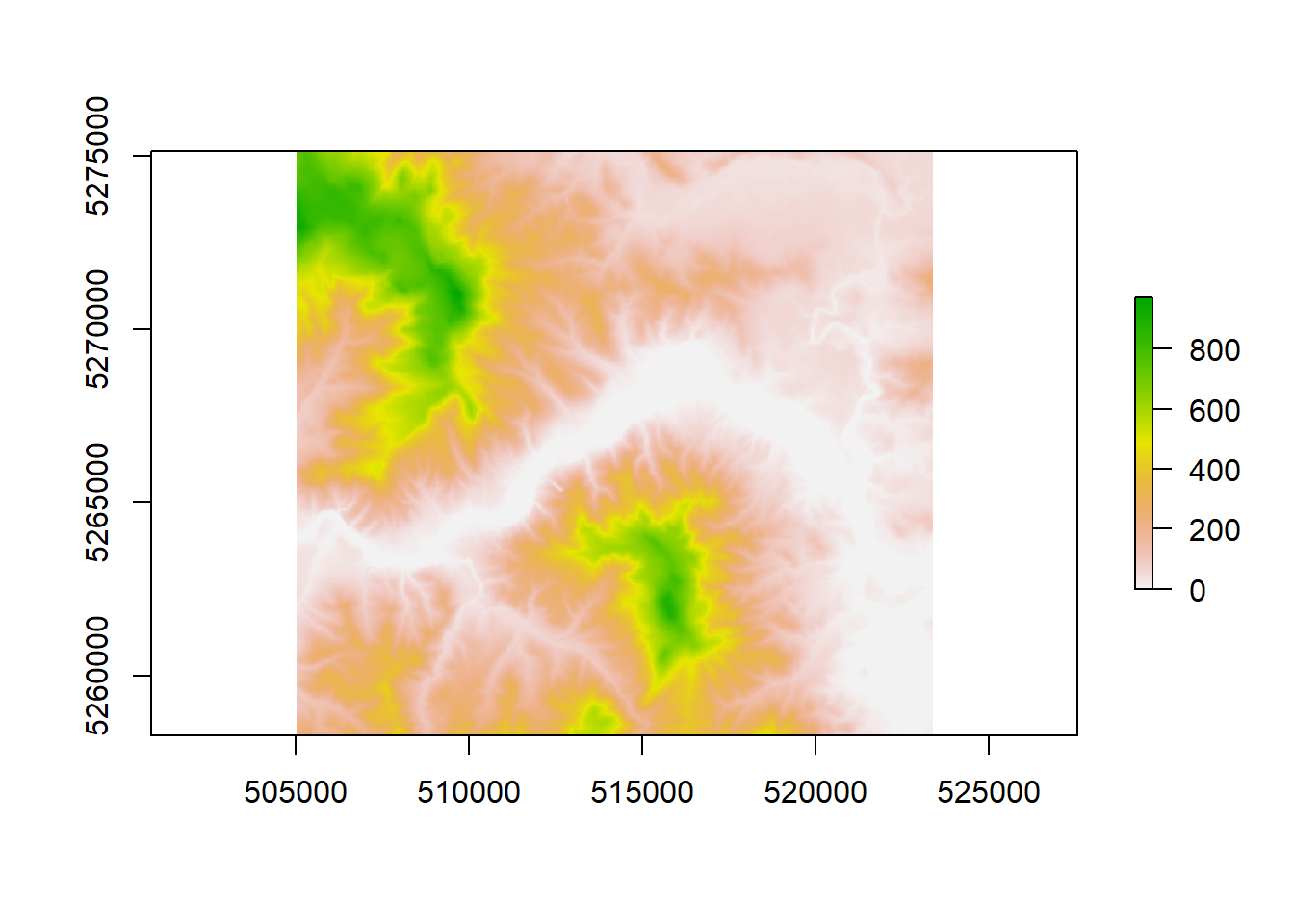

To work with *rayshader** we will need to transform this to a matrix with the raster_to_matrix() function. Then we can start with add a specific texture as well as shadows.

elmat = raster_to_matrix(localtif)
elmat %>%
  sphere_shade(texture = "desert") %>%
  plot_map()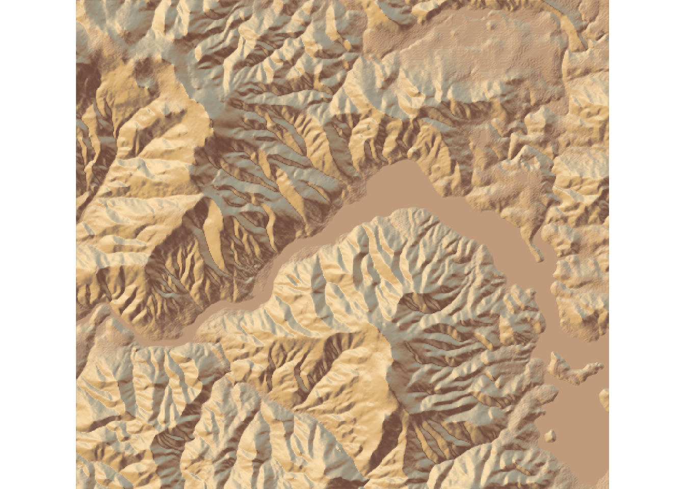

The shadows are computed for a default sun angle, but we can change that angle if we like.

elmat %>%
  sphere_shade(sunangle = 45, texture = "desert") %>%
  plot_map()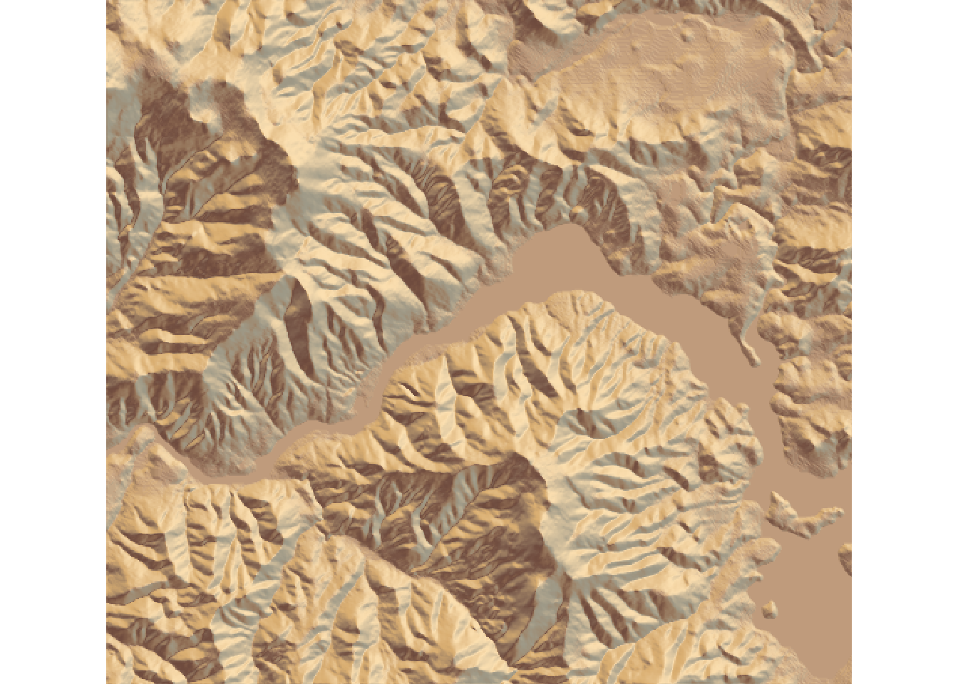

Now you might have noticed that the areas in the valley look suspiciously flat. That’s because they are water surfaces. With the two functions detect_water() and add_water() we can add water to our map. detect_water() returns a binary matrix with the same dimensions as elmat. A one indicates that the corresponding cell in elmat contains water and a zero that the cell does not. With the cutoff argument you can specify how high the water should be, i.e. which cells are classified as carrying water. High values mean lower water level.

elmat %>%
  sphere_shade(texture = "desert") %>%
  add_water(detect_water(elmat, cutoff = 0.9), color = "desert") %>%
  plot_map()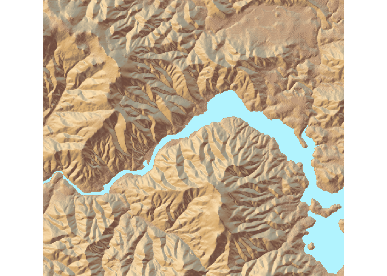

Now we don’t have any shadows on the water yet. But that can be done with add_shadow().

elmat %>%
  sphere_shade(texture = "desert") %>%
  add_water(detect_water(elmat), color = "desert") %>%
  add_shadow(ray_shade(elmat), 0.5) %>%
  plot_map()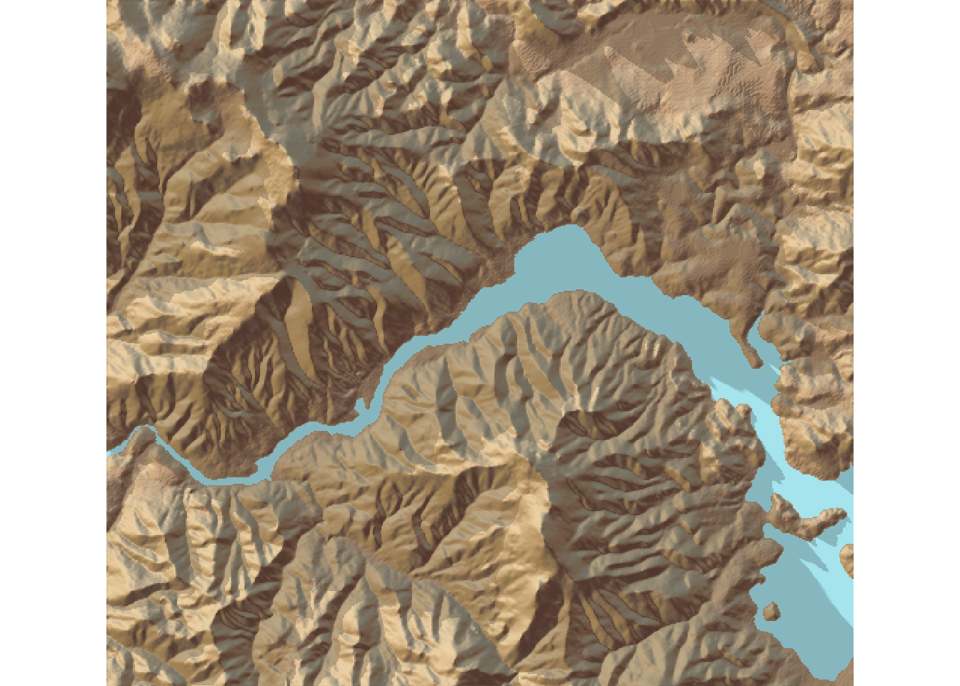

In addition to rayshade we can also ad ambient shade, to make it look even better.

elmat %>%
  sphere_shade(texture = "desert") %>%
  add_water(detect_water(elmat), color = "desert") %>%
  add_shadow(ray_shade(elmat), 0.5) %>%
  add_shadow(ambient_shade(elmat), 0) %>%
  plot_map()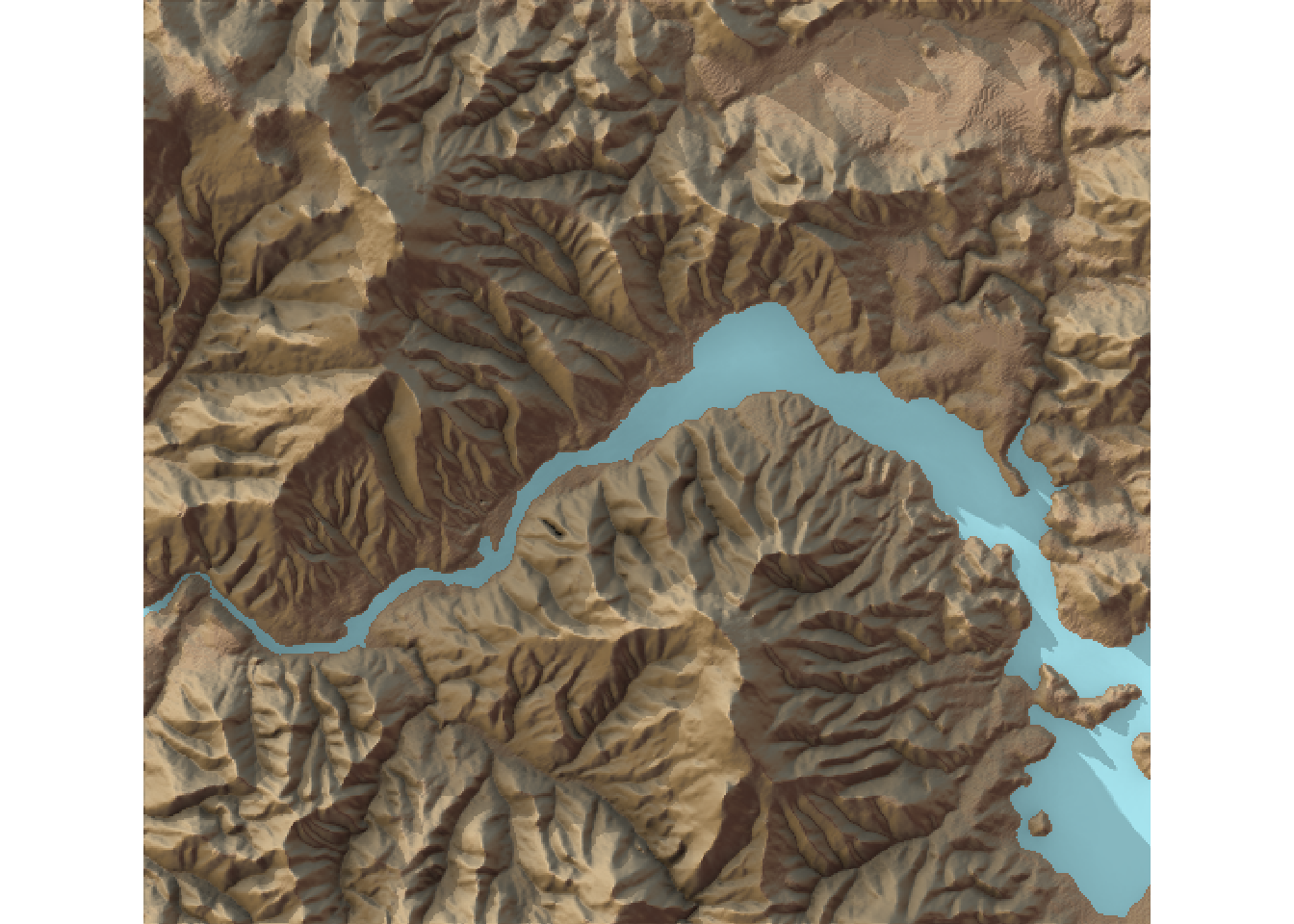

All this was only the preparation though for the 3D capabilities of rayshader.

elmat %>%
  sphere_shade(texture = "desert") %>%
  add_water(detect_water(elmat), color = "desert") %>%
  add_shadow(ray_shade(elmat, zscale = 3), 0.5) %>%
  add_shadow(ambient_shade(elmat), 0) %>%
  plot_3d(elmat, zscale = 10, fov = 0, theta = 135, zoom = 0.75, phi = 45, windowsize = c(1000, 800))
Sys.sleep(0.2)
render_snapshot()