R package of the week: DataExplorer
install.packages("DataExplorer")
library(DataExplorer)
data = readRDS("collected_site_scores.RDS")
This weeks package is similar to last weeks. Just like xray Seibelt (2017), DataExplorer Cui (2020) is used for exploratory data analysis. To highlight the features and capabilities of the package we will use a data set of different diatom metrics derived from a large data set of diatoms, which I unfortunately am not able to share with you. These metrics were computed with the diaThor package, which I will cover in a later post.
How do my data look?
Assume you just got this data set and now you want to get a feeling for it. Your initial questions might be: Are there any missing data?
plot_missing(data)
Indeed, 100 rows in epid are missing which constitutes 4.4% if the rows. What about our categorical variables. How are they distributed?
plot_bar(data)## 1 columns ignored with more than 50 categories.
## gr_sample_id: 2285 categories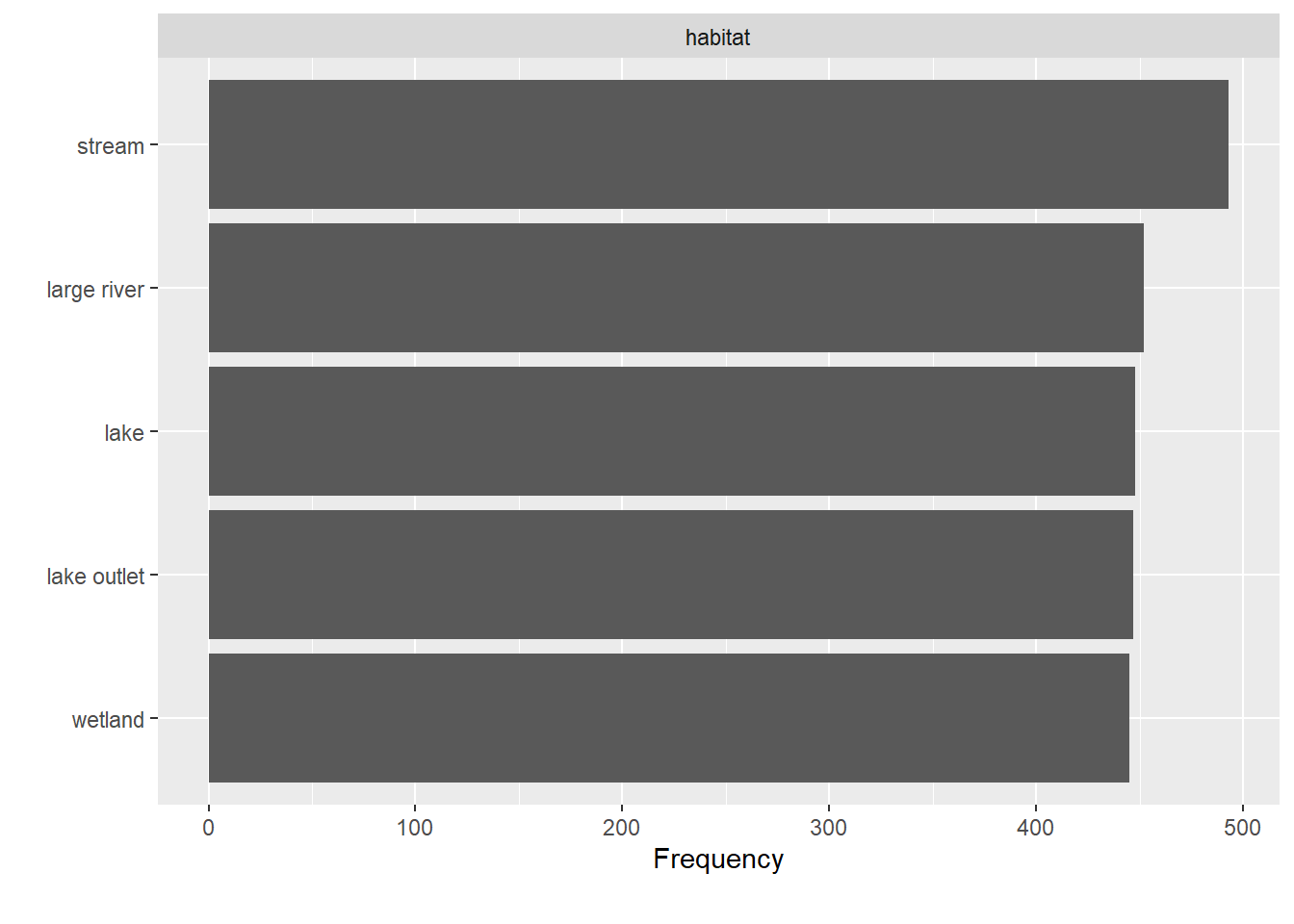
Note that I did not have to tell the function which variables are categorical.
As long as they are formatted as a factor, the function will pick them out itself.
Of course, we also want to know how the continuous variables are distributed, which we can find out with plot_histogram().
plot_histogram(data)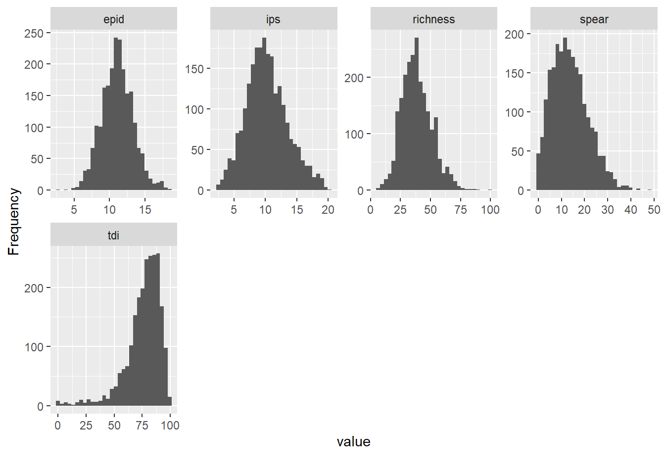
Relationships between variables
Now we have a basic understanding of all the variables we can start to look at relationships. All metrics except for richness are diatom indices. This is not the place to go into details but diatoms are great as bioindicators, i.e. to judge the state of a waterbody. There are many different species (according to Smol and Stoermer (2010) about 200 new species are described each year) and many of them are sensitive to environmental conditions. These indices (EPID, IPS, TDI, SPEAR) are different ways to achieve this goal. They focus on somewhat different aspects of the environment. Actually SPEAR is distinct from the others, it gives the relative richness of species that are sensitive to pesticides and was originally developed for invertebrates. Wood et al. (2019) applied the approach to diatoms. Anyhow, are these metrics depended on the species richness?
plot_boxplot(data, by = "richness")## Warning: Removed 100 rows containing non-finite values (stat_boxplot).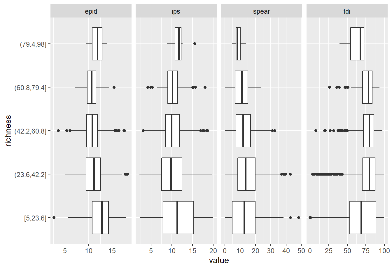 No actually it does not look like it.
As alternative to the boxplot, we could also have looked at scatter plots
Because the data set is quite large (2285 observations) we will only look at a subset of 100 rows (sampled_rows)
No actually it does not look like it.
As alternative to the boxplot, we could also have looked at scatter plots
Because the data set is quite large (2285 observations) we will only look at a subset of 100 rows (sampled_rows)
plot_scatterplot(dplyr::select(data,!gr_sample_id) , by = "richness", sampled_rows = 100)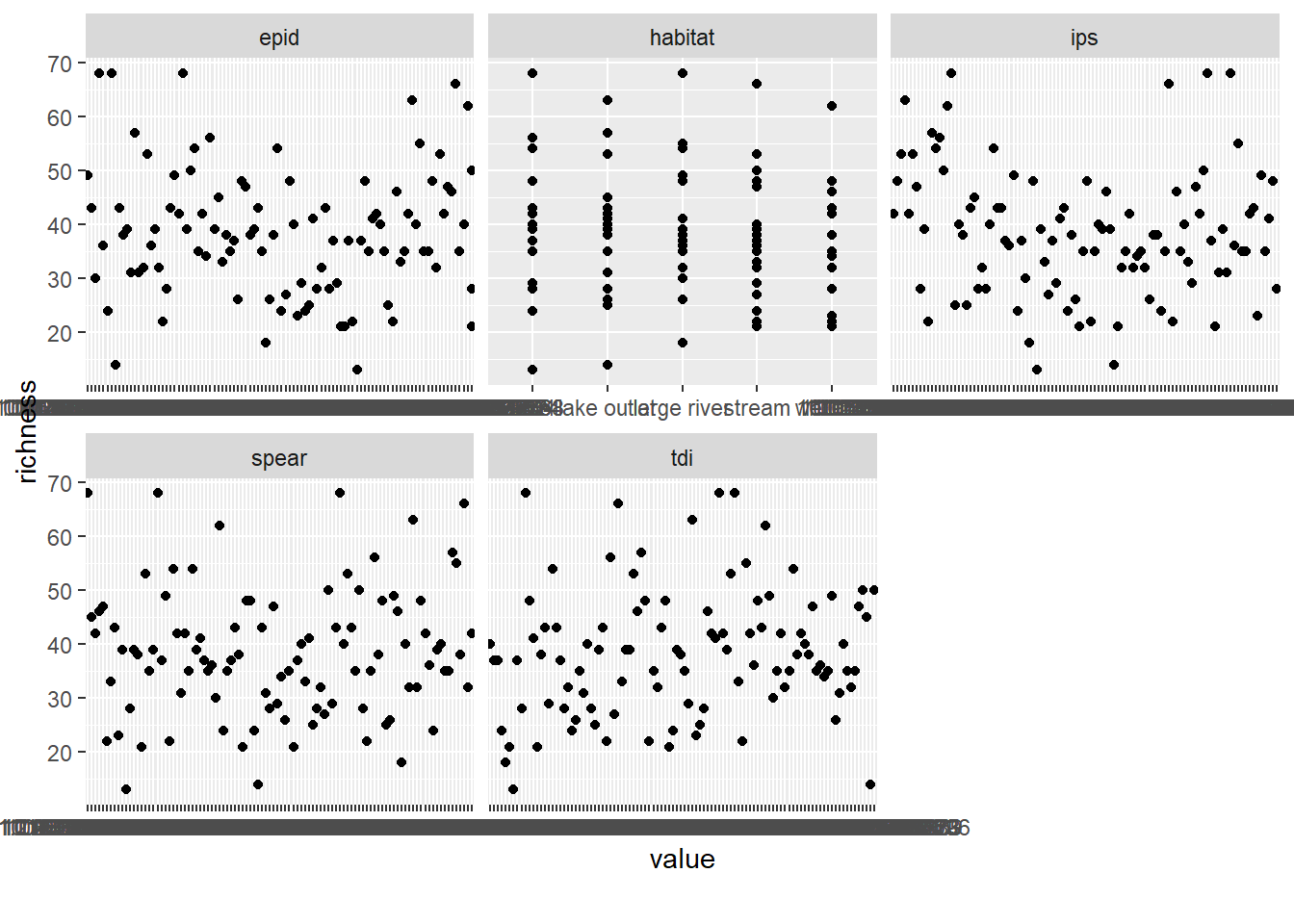
In practice we should either plot all data, or repeat the step above several times to ensure that the random selection of sites does not impact verdict. However in this case there does not seem to be any correlation between species richness and any of the diatom metrics.
As a last step we can look at the correlation plot for the variables.
plot_correlation(data)## 1 features with more than 20 categories ignored!
## gr_sample_id: 2285 categories## Warning: Removed 18 rows containing missing values (geom_text).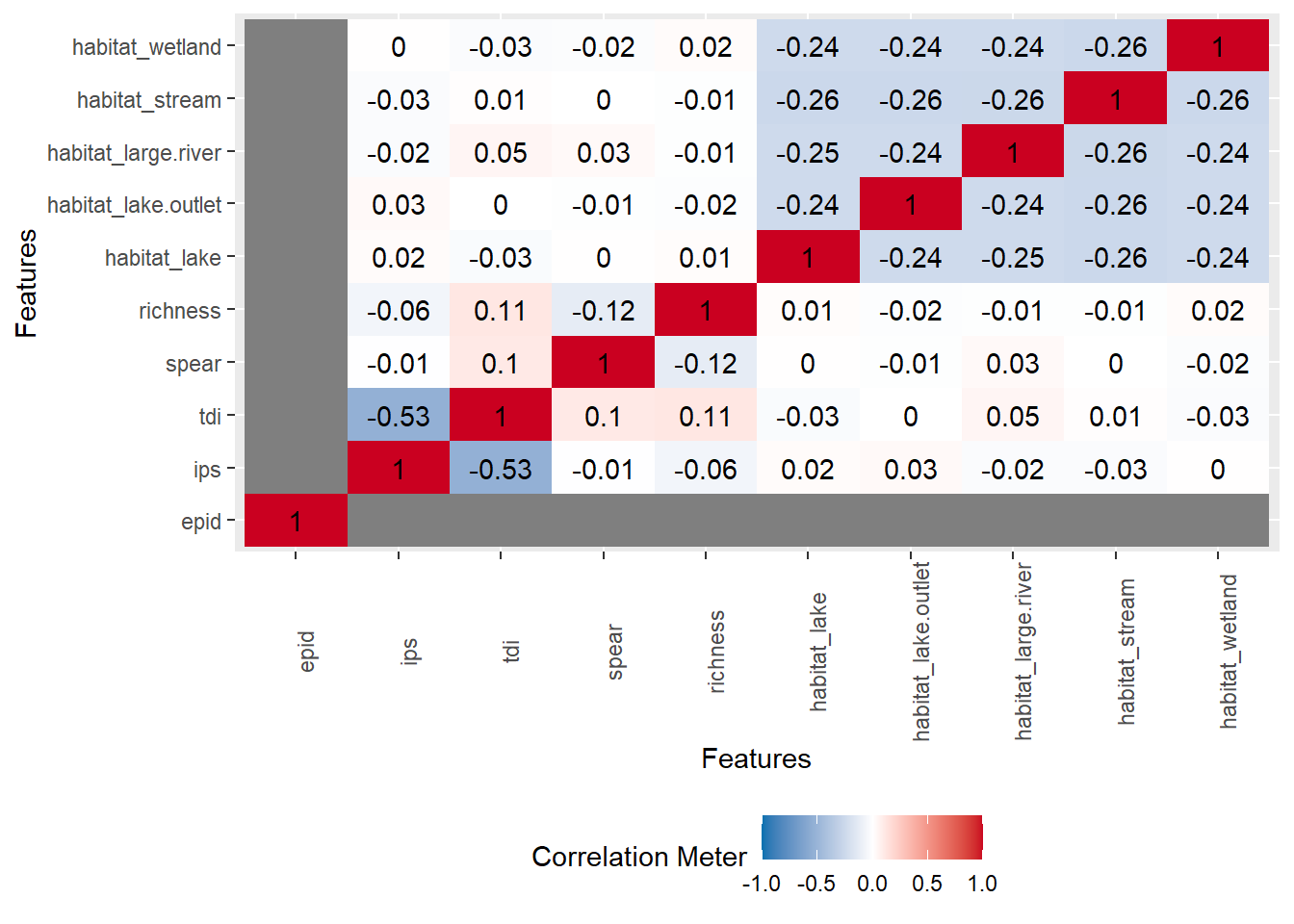
For the lazy data explorer
Another nice feature is the create_report() function, which allows you to kick back for a moment while the function automatically runs several of the functions above as well as QQ-Plots and a PCA on the data set and compiles a HTML document with all of them.
create_report(data)